Real-Time Smoke Simulation
and Visualization
1. Introduction
This directory contains
the code for the Real-Time Smoke Simulation and Visualization assignment. The
code contains a real-time simulation of matter which flows under the influence of
a user-controlled force field. The simulation follows the Navier-Stokes
equations for fluid flow. This document describes briefly how to compile the
code and the structure of the main program. This is not intended as an in-depth
description of how to write or compile programs in C or another programming
language, OpenGL, event-based programming, or how to build a real-time fluid
simulation engine. However, starting here, you should be able to compile the
code and add visualization features to the provided skeleton application.
2. Structure of the code:
The
provided software consists of three main parts:
·
a mathematical library, called
FFTW (standing for Fastest Fourier Transform in the West), is used to provide
the numerical engine that simulates a fluid flow in two dimensions.
·
the GLUT library (GL Utility
Toolkit), used to provide simple OpenGL graphics, mouse, and keyboard support
to the application.
·
a very simple application skeleton
which shows how to call the FFTW simulation code, steer it interactively
using the mouse, and do some basic visualization and graphics, using GLUT.
All the
code is written in the C programming language. Although it helps if you
understand C, you should be able to rewrite the application skeleton to use the
FFTW library from the programming language of your choice (e.g. Java, Python)
The
provided code is structured in the following main components (files and folders):
·
fftw-2.1.3: Contains the
sources of the FFTW library
·
fluids.c: The
application skeleton which calls the FFTW library
·
GLUT: Contains the
GLUT (GL Utility Toolkit) library
There are
some other less important files and folders. These will be described in the
building instructions below.
3. Building the code
Let us
first assume you have a C compiler installed (e.g. Microsoft Visual C++ Express
Edition, or GNU gcc, both which are freely
available). To build the application, you have to compile all C files in fftw-2.1.3/fftw,
fftw-2.1.3/rfftw, and fluids.c in a
single executable, and link with the GLUT/glut32.lib.
If you have
the Microsoft Visual C++ compiler, you can compile by simply opening the Smoke.sln solution file and building it – either in debug or release mode.
The
following directories contain Visual C++ project-related files:
·
FFTW: Contains the
project for building the FFTW library
·
Smoke: Contains the
project for building the complete application
·
library: Contains
the FFTW static library FFTW.lib that the application
is linked against.
The final
application, Smoke.exe, is created in the top-level directory. Note
that, to run it, you must have the GLUT library glut32.dll in the same
location as the executable. This library is provided with the code.
Of course,
you can build the code using different C compilers.
4. Running the code
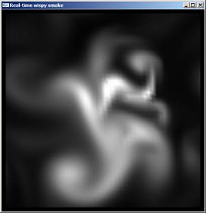
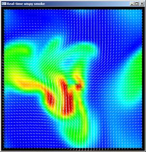
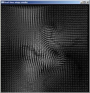
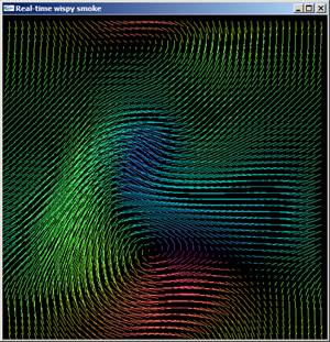
Just run
the smoke.exe application. You will get a text window showing some help
messages and a graphic window. Select the graphic window. To control the
simulation, click and drag the mouse. To change the visualization and/or
simulation options, press use the indicated keys in the graphical window. After
a bit of experimenting, you should be able to create some images like the ones
shown below:
5. The application
The main
application is a single file, fluids.c. The
structure of this file is described briefly below. See also the comments
embedded in the source code. The purpose of these explanations is to help you
understanding how you can start modifying the code, to add new visual
functionality to it, or how you can start porting the code, if you want to
write your assignment in a different programming language than C or C++.
As a
general note: Do not worry too much if you do not understand the numerical
code. This is not the purpose of the assignment. You can use that code as a
simulation ‘black-box’. The purpose is to focus on building new visualization
methods atop of that simulation code.
A list of
the most important data structures and functions in the program follows. The
functions are divided into three groups: simulation, visualization, and
interaction. They are listed in inverse order of importance to the program’s
functionality.
Global
data structures:
·
plan_rc, plan_cr: The 2D uniform n*n grid on which the
simulation takes place. The actual data type for these structures comes from
the FFTW library – you do not have to use these directly.
·
fx, fy: The components of the 2D force
vectors that drive (steer) the simulation. These are directly controlled by the
user via the mouse.
·
rho,rho0: The density of the matter which flows in. As
the flow direction and speed changes, so does the density. See below.
·
vx,vy,vx0,vy0: The components of the 2D velocity field which is
simulated. The simulation computes v,rho
(velocity and density) out of v0,rho0 (their previous values one
time-step ago) and f (the forces).
In
a functional notation:
(vx, vy, rho)
= do_one_simulation_step(vx0, vy0, rho0, fx, fy)
or in a more mathematical notation
(bold denote vectors):
(v (t+Dt), rho(t+Dt))
= do_one_simulation_step(v(t), rho(t), f(t+Dt))
Simulation
functions:
·
do_one_simulation_step: Does one single step of the fluid
flow simulation. This involves passing the mouse-controlled forces to the FFTW
library, executing one simulation step to compute the new velocity and density
values, and visualizing all these.
This function is called repeatedly to keep on
the simulation running forever. This is the first of the two functions
calling the FFTW library.
·
solve, diffuse_matter: These functions contain the actual
numerical simulation code which computes vx, vy, rho out of vx0, vy0, rho0,
and fx, fy.
·
init_simulation: Initialize the various global data
structures as function of the grid size. This is the second of the two
functions calling the FFTW library.
Visualization
functions:
·
visualize: Contains all the visualization code
which draws the velocities vx,vy, and the density rho. This is the main visualization function.
·
rainbow: Maps a floating-point value to a RGB
color using a blue-to-red (rainbow) colormap.
·
direction_to_color: Maps a vector’s direction to a RGB color using a directional hue-based colormap.
Interaction
functions:
·
main: The main program. Prints some help
messages and sets up GLUT to perform the display and interaction.
·
drag: Called when the user
clicks-and-drags the mouse in the visualization window. This sets up the force
(fx,fy) and density (rho) at the mouse location, effectively steering the
simulation.
·
keyboard: Changes
the simulation and visualization parameters based on keyboard input.
·
display: Draws
a new visualization frame, whenever the simulation is ready with producing a
new step.
6. Further reading
If you are interested
to study the above topics in more depth, there is additional documentation in
the fftw-2.1.3 directory on the FFTW library implementation. The overall
simulation algorithm is described in the paper “A Simple Fluid Solver based on
the FFT” by Jos Stam
(Journal of Graphics Tools, volume 6, number 2, 2001, pages 43-52). You can
find the paper online e.g. at http://www.dgp.utoronto.ca/people/stam/reality/Research/pub.html
or other sites (Google for it).